Viewing and Printing Spreadsheets
View the Spreadsheets
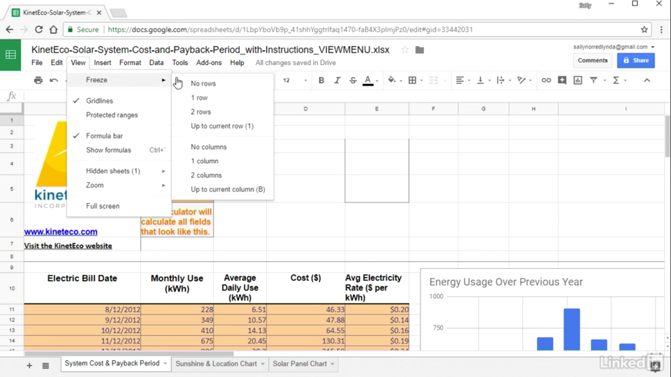
To access the View menu, click the word view in the upper menu above the Google Sheets toolbar. You’ll see a dropdown menu appear with several options listed.
- The first option is freeze. This refers to freezing rows or freezing columns in your spreadsheet view. Freezing rows and columns are useful if you want to keep a row or column header label visible as you scroll through a large spreadsheet.
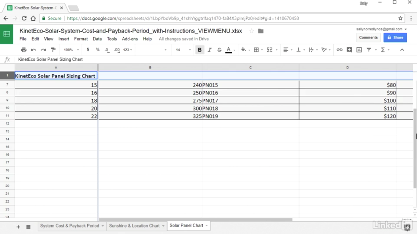
- You can freeze a single row or column, or multiple rows, or multiple columns, or even rows and columns at the same time. If you want to freeze the top row of this spreadsheet. I select the row, click the view menu, and click freeze one row. Then when you scroll through the spreadsheet, you can still see that top row. You can unfreeze this row or columns by clicking view, freeze, no rows or columns.
- For example :
—————————————
Formula bar :
————————————–
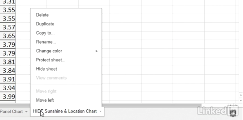
Hidden sheets :
——————————————–
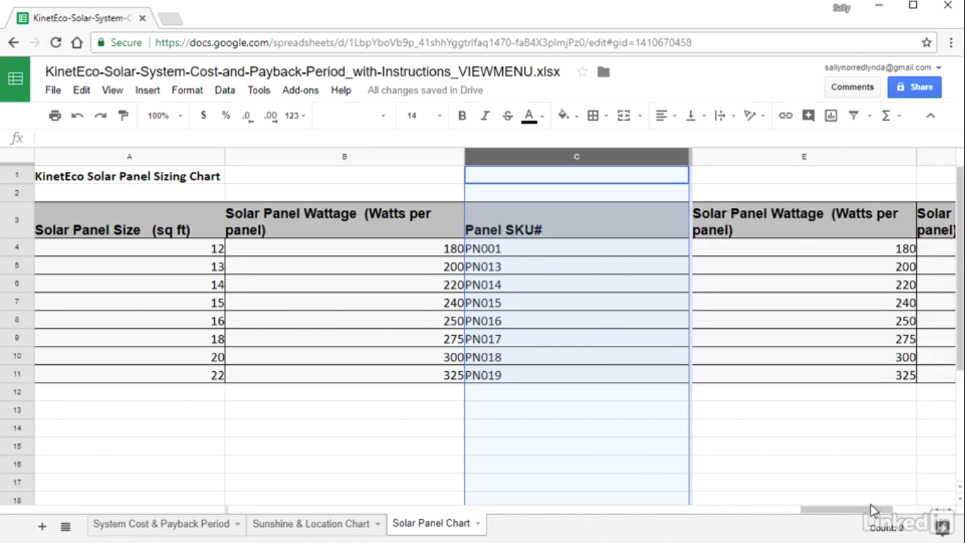
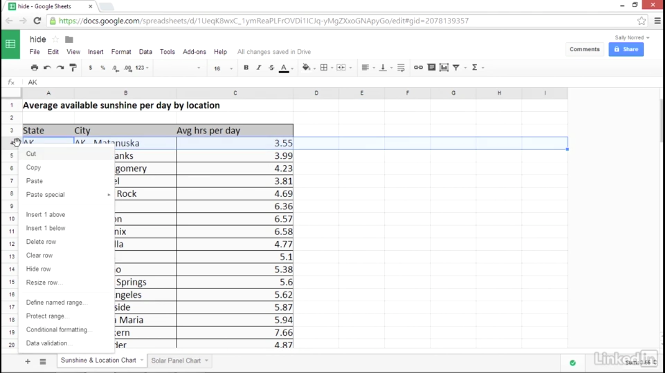
Hidden Column & Row :
- You have to right click then select hide row or column
————————————————————-
Publishing a spreadsheet to the web
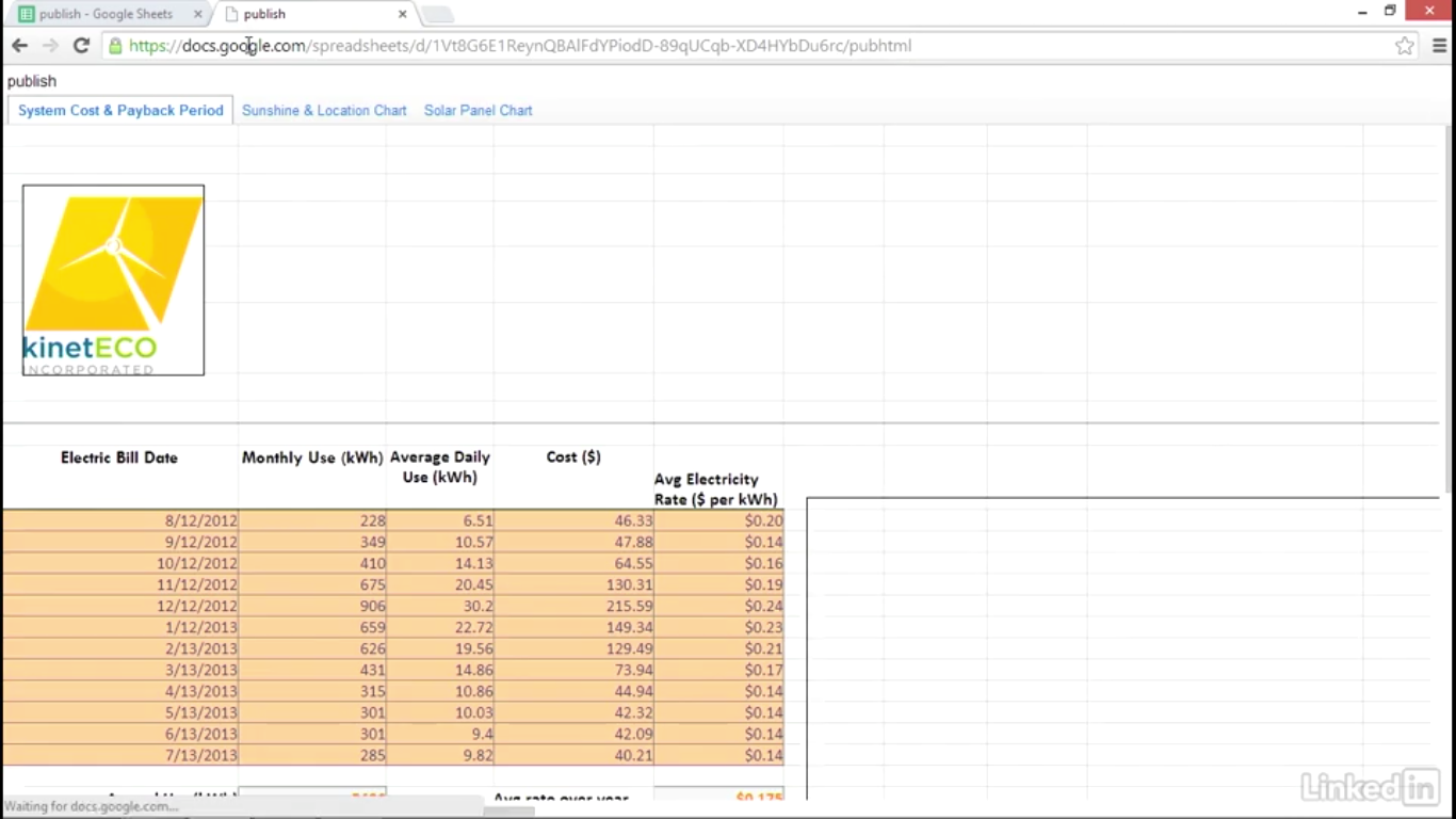
- Google Sheets allows you to publish your spreadsheet to a web page with a single click. Publishing your spreadsheet to the web allows you to share your spreadsheet for viewing with the URL address. Once it’s published on the web, it’s publicly accessible. The other will only be able to view the spreadsheet from the shared URL. They will not be able to edit or revise the published spreadsheet.
- How to do this?
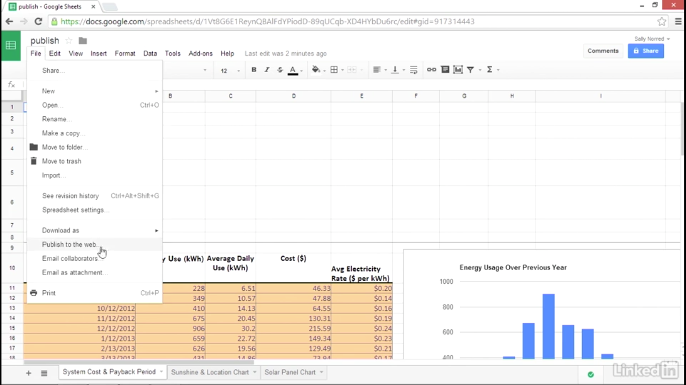
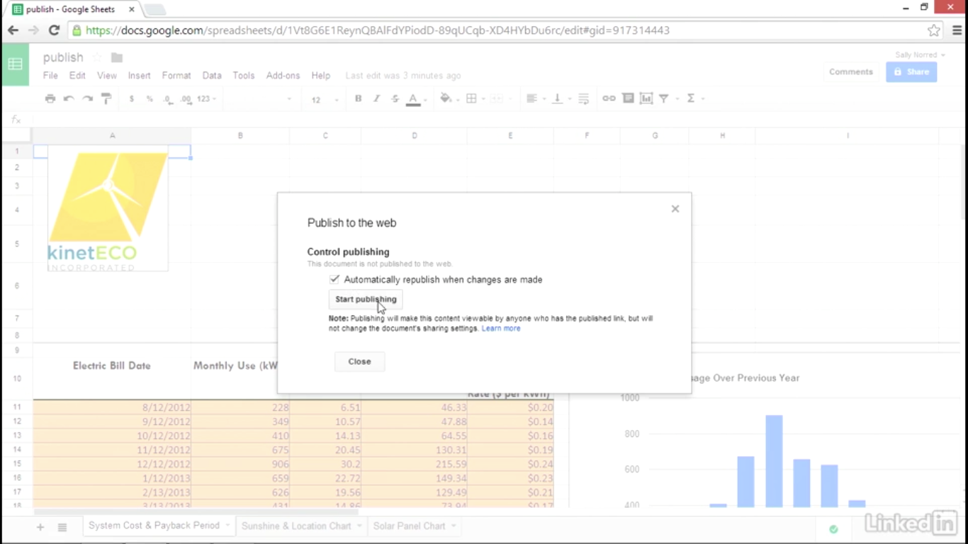
Click file for the menu and select publish to the web. Keep the automatically republish when changes are made check box checked if you’d like to keep the revisions in sync with the published version. Then click the button labeled start publishing. Click ok to confirm.
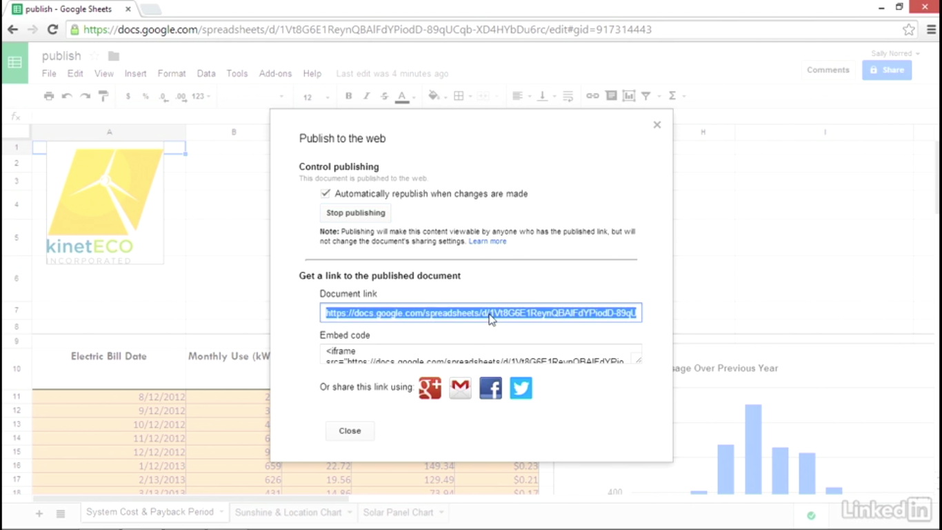
Link :
- To turn off publishing and remove the spreadsheet from the web, click the stop publishing button. Click ok to confirm. The spreadsheet will be removed from its web page location.
—————————————————————-


