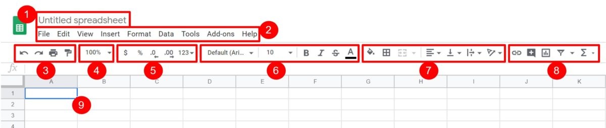
1. Spreadsheet name
2. Menu bar
3. Basic controls (undo, redo, print, format painter)
4. Zoom
5. Number formatting options
6. Text formatting options
7. Cell formatting options
8. Advanced controls and functions
9. Active cell

Formatting Cell, Row, and Column Data 

(Use Format on Menu bar, Number Formatting Option, Text Formatting Option, & Cell Formatting Option)

For numbers, you can select between a simple decimal, percent, dates, currencies, and many others. You can also increase or decrease the number of decimal places displayed using the main toolbar. Note that this doesn’t change or round the real value, just the number displayed.

For normal text, you have the standard options for bold, italic, underline, and strikethrough, as well as font types, font sizes, and alignment. Cells themselves can be formatted as well. You can change the background color, merge or unmerge cells, or add borders.

To speed up your formatting, you can also select an entire column or row by clicking on the letter or number at the top or left of the screen.

You can merge your cell in your spreadsheet. All you need to do is select more than one cell and click the merge icon in the upper middle of the toolbar. The icon has two arrows pointing together, and it’s greyed out unless you have more than one cell selected.

You can also wrap text on your cell, just select your text on one cell and click the wrap icon

Formatting Tips 

(Use Basic Controls Menu)

If you want to copy the formatting of one cell to another cell, just click the paint format icon on the basic controls menu and click and drag to the select cell. Or you can use Ctrl+Y on your PC keyboard or Cmd+Y on Mac keyboard.

Using Conditional Formatting 

(Use Format on Menu Bar)

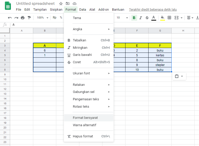
For example, you want to see any item on the list where the number is greater than 8. First, select the column of the number and then click the menu like on the picture.

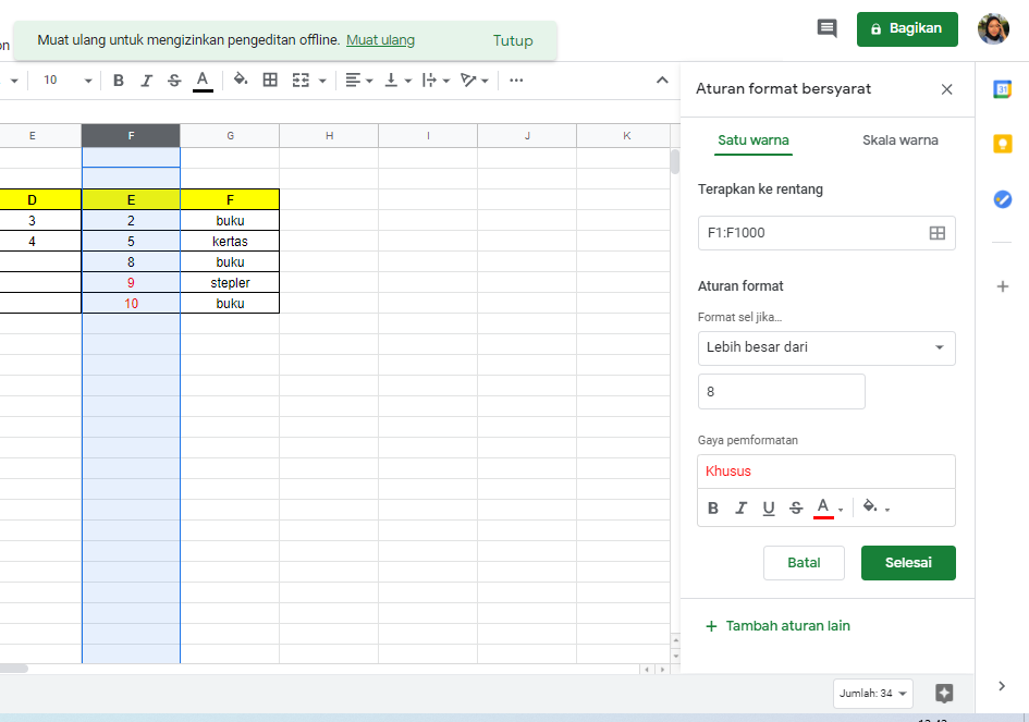
Create a rule, greater than 8, and format the text color, also you can format the text background if you want. and click finish. And you can see the numbers where greater than 8 are red.

You can use another menu of conditional formatting in the same way. See the picture below:

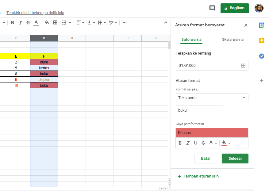
Notice, if you change one of the cells in the range to “buku”, it automatically highlights as well.

And if you want to check the type of your item on column G, and change the formatting in the type, column E, accordingly. Highlight the column where will be adding the formatting (column type), and use the format like the picture below:

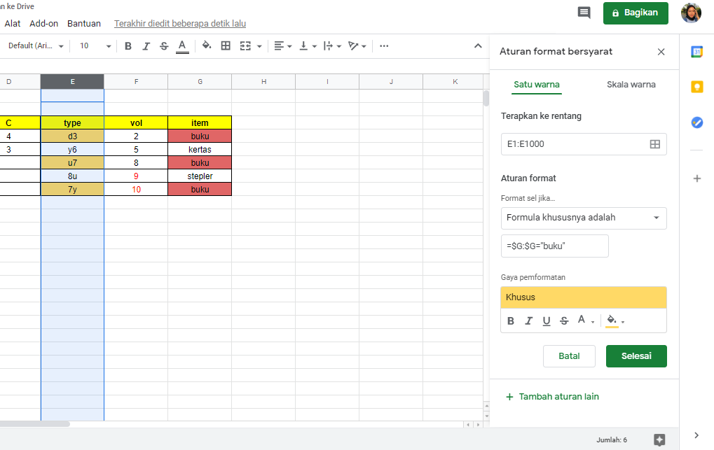
Use the custom formula, so you know that the type in column E represents a type of the “buku” in column G.

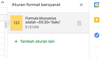
To remove a rule, just click the column, go to conditional formatting, and click the trash logo like the picture below:

You should also know, if you copy and paste from the cells or range that has formatting rules, these rules will be applied when you paste the copied data.

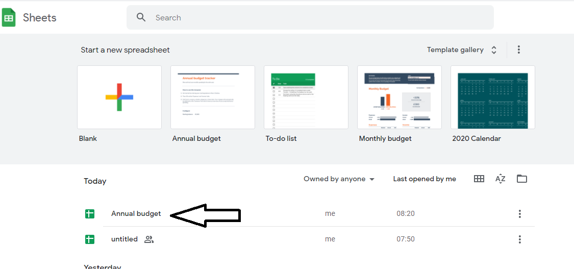
Creating a Spreadsheet from a Template

To go back to your sheets home and you can see any recently accessed files 30 days and beyond.

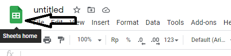
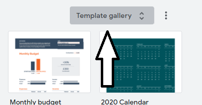
You can create a new blank spreadsheet or search for an existing sheet. Click the template gallery button will bring up many more templates that you can use to start your project.

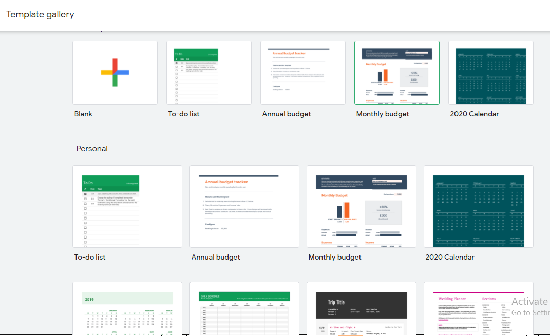
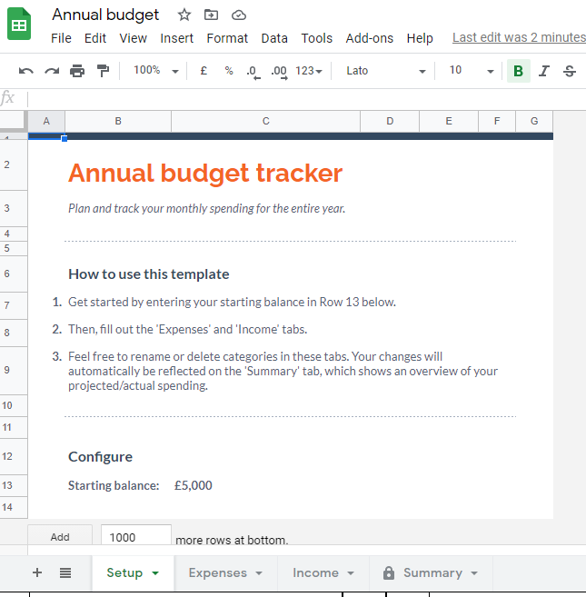
For example, click Annual Budget, it’s going to open up pre formatting spreadsheets.

If you’ve been working on this for a few minutes it will save this document.